Example 1: Exponential growth 

The simplest GEM we can build is one for exponential growth. The standard ODE for this is  , where the rate of change in the population size N is proportional to population size with an intrinsic rate of increase r. Implicit in r are births and deaths, and because GEMs require birth and death events, we must rewrite exponential growth as . The events in this model come from the two rate terms, bN and dN. In this first GEM, we will focus on the evolution of the birth parameter itself rather than on some trait that is linked to births, so we don’t need to specify a trait-parameter link.

The steps we need to get through are:

1. Initiate some empty vectors to hold stuff
2. Decide on some key information such as trait mean, amount of variance, and heritability
3. Make an initial trait distribution to start the population
4. Pick an individual
5. Determine event probabilities
6. Choose an event
7. Update population trait distribution
8. Continue steps 3-6 until the desired amount of time has passed
9. Summarize the resulting trajectories

Download the entire exponential growth GEM along with necessary associated files below, but I will go over a few key lines of code here first:

Picking individuals at random.—On line 28 below is this bit of code:

x_dist_init = pick_individuals(b,cv*b,R(1));

In the zip folder download, you will find a function called ‘pick_individuals’. This function has the algorithm we use to pull individuals at random from a lognormal distribution with mean b and standard deviation cv*b. You could use other distributions, but most traits cannot be negative and thus are more likely to follow a lognormal distribution than a normal one. In its first use on line 28, we are picking R(1) individuals, which is the population size at the start of the run. Later we will use this same function to pull single individuals that are added to a population upon a birth event.

Picking an individual for events.—On lines 36-37 is this code:

whosnext = randi(size(x_dist,1),1);
x_next = x_dist(whosnext);

These lines just randomly choose an integer (randi) from the size of the distribution (=population size). We use ‘size’ specifying the number of rows (the ‘,1’) rather than length because you can have introduce a matrix of traits instead of just a vector of one trait. The element identity (row of the distribution) is used to pull a value of the trait from the distribution of traits (x_dist) and renamed ‘x_next’, which is what will be used to influence events in the next event. In this first model, we are focusing on births (b). Births is a parameter in our model so it needs no trait-parameter link, but if you were connecting births to a trait (such as clutch size or something), this is where you would write that trait-parameter link.

Determine event probabilities.—You can see the rate terms on lines 42 and 44, and below on lines 47-50 is where the event is chosen:

CS_vector = cumsum([b_R d_R]);
Slice_widths = CS_vector./CS_vector(end);
LI = rand < Slice_widths;
Event_index = find(LI,1,'first');
 
The steps here are as follows. The ‘cumsum’ function adds up all the terms so that the total sum of terms is the last element of the vector CS_vector. We then divide that vector by that last element to get probabilities across all the terms. LI is a list index of 0s and 1s where a 1 indicates that the random number generated by ‘rand’ is less than the corresponding elements in ‘Slice_widths’. Then the final row picks the first of these elements that are a 1, and that element corresponds to the event that happens.

Updating the populations.—On lines 53-60, events transpire based on the Event_index. This index is just an integer that specifies which event happens from the list determining the CS_vector. They can be in any order, but the code follows the order specified on that line. If the event is a death, we just remove the participating individual from the trait distribution (line 59). If the event is a birth, we then need to pick an individual following the rules for determining the potential trait. See DeLong and Luhring (2018) for more details on this, but the short version is that the mean of this potential distribution is the heritability-weighted average of the parent and the initial mean, and the standard deviation is the heritability-weighted average of the current and initial distributions. This individual is then dropped into the distribution at the end. After either event, the length, mean, and variance of the trait distribution vector is used as the new current population size, mean trait, and trait variance (lines 62-64).

Updating time.—On line 66, time is advanced by an increment determined by an exponential distribution for the total of the rates in the model.

Summarizing results across replicates.—There is code before and after the GEM loop that picks out information at consistent times across replicates. These values can then be used to find median trajectories with some confidence bounds. This example uses the middle 50% of observations as an indicator of variability (lines 83-84).

To run this GEM, download the zipped folder here. This folder contains the GEM file itself, a script to run it and plot the outcome, the ‘pick_individuals’ function, an exponential growth model file, and a plotting function I like called jbfill. Save all these functions into the same folder and run the script called ‘Run_EG_GEM_intro’.

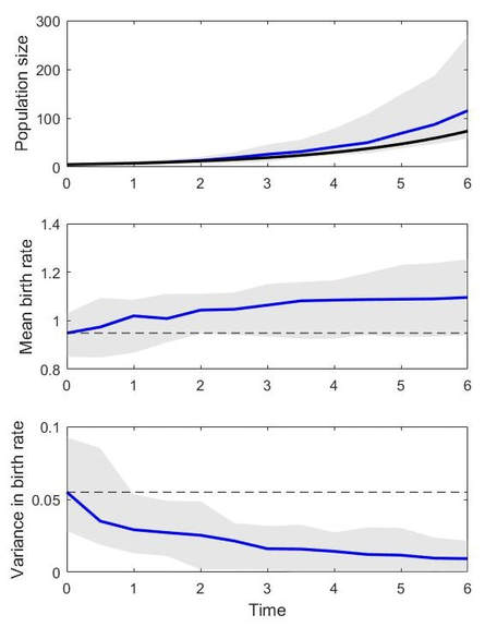
When you are done, you should have something that looks like the figure below. In this figure, the ODE solution is plotted as a thick black line, the median GEM outcome is plotted as a thick blue line, and the middle 50% of GEM simulations are plotted as a shaded gray area. The dashed lines show starting conditions. This figure shows that the GEM produces selection favoring higher birth rates (which makes sense), accelerates population growth as a result (the expected eco-evolutionary outcome), and erodes variance through time (also as expected). This example has a cv of 0.3 and heritability of 1. Remember that evolution requires heritable trait variation, so if you zero out either the cv or the heritability, evolution will not happen. You can try this just by changing these levels in the code (heritability on line 11 and cv on line 12) and rerunning the script.

It’s also worth pointing out that the stochastic nature of GEMs means that you can get quite different outcomes when you choose too few replicates. My rule of thumb is that you should run enough replicates that the outcomes pretty much look the same each time. The one shown below was run with 50 replicates – that’s probably not enough but it usually looks about like what you see here.